
Truth be told, I have a love hate relationship with mean (not the word mean, I mean the mean the average). Ever since I started my PE journey, the mean is always there, it’s pure, it’s simple yet so deceiving. Statistically, the observed difference in mean could happen by chance, i.e. A and B are not different statistically.
Picture this typical setting: you, as a rising star engineer, had your boss’ blessings on a new R&D escapade. Budget? Check. Support team? Check. Time to test the waters with your new tech toy (let’s call it Gizmo B) versus the old faithful (aka Clunker A). But here’s the million-dollar question: “Is Gizmo B really outshining Clunker A, or is it just burning cash faster than a rocket?” Instinctively, we (petroleum engineers) plunged into the data abyss, hoping to fish out some golden insights. However, finding a clear winner in every scenario is as rare as spotting a unicorn.
Let’s enter the world of statistical modelling and hypothesis testing. In this example (disclaimer: all data had been masked), I compared A and B.
First up, the histogram face-off: Gizmo B vs. Clunker A. The observed difference in mean is 66 Mstb. Visually, there was not much difference between them. In addition, “difference between average values of B and of A” can not be interpreted as “the average difference between observed values of B and of A” (take a deep breath…). This is a common misinterpretation when we perform economic justification.
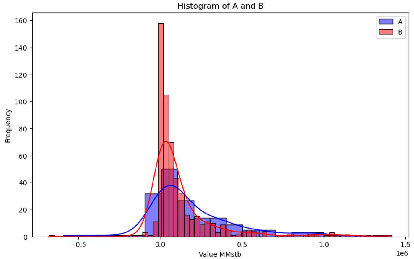
Histogram Face-off
Next, I built a statistical model on difference in means using Bootstrap method. The histogram below showed B was indeed a clear winner
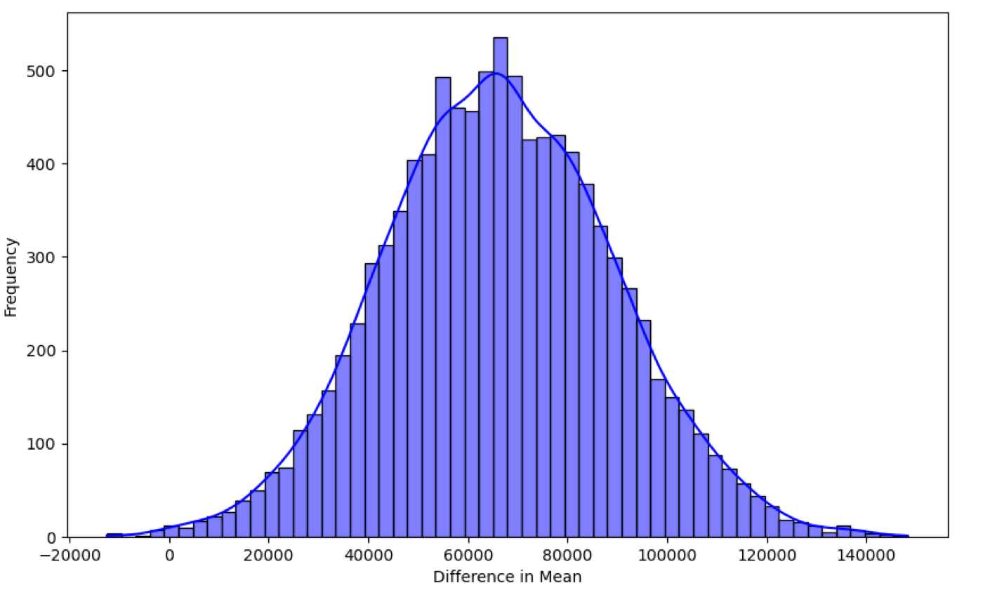
Bootstrap Method
🥳The verdict: beyond our means
So, dear my O&G network, it’s not just about living within our means, but understanding what those means truly reveal (or conceal). Here’s to unearthing truths, one bootstrap at a time!
#BeyondTheMean #AdvancedStatisticalTesting #Bootstrap