
As engineers, we often find ourselves engrossed in the depths of process data. And yes, it’s no secret that more often than desired, we encountered data anomalies, often blamed on faulty instruments. But what if the instruments weren’t the culprits?
Take, for instance, a gas plant I once observed:
- Inlet Meter (A) with a typical value of 150.
- Outlet Meter (B) with a typical value of 149.
- Plant Usage/Wastage Meter (C), expected to be A - B, so a typical value of 1.
Each meter had been calibrated to a precision of +/- 1%. Yet, when executing a mass balance, I was consistently confronted with an error that was hard to justify. Despite multiple recalibrations and the fundamental equation being sound, the puzzle remained unsolved.
Enter the realm of Error Propagation—a cornerstone in many STEM fields. It sheds light on how errors disseminate through sequential mathematical operations. Before you panic, I promise I won’t drown you in complex mathematical jargon. Instead, let’s decipher the mystery using simplified approaches.
Analytical Method:
- Establish bounds for A (148.5, 151.5) and B (147.51, 150.49).
- Calculate the bounds for A-B:
- Upper bound: 151.5 - 147.51 = 3.99
- Lower bound: 148.5 - 150.49 = -1.99
Voilà! The discrepancy is evident. The computed (A-B) error shoots up to +/-200%, while the observed meter C maintains an error of just +/-1%.
But here’s another intriguing question: What are the odds that the (A-B) value would deviate from the expected range of (0.99, 1.01)?
Enter the Monte Carlo Method—a technique that portrays the (A-B) distribution based on various A and B distributions. For our example, we’ll consider that the errors in A and B are uniformly distributed between their respective bounds. Using Python, the simulation’s outcome is shown below. Surprisingly (or not) it’s a rare occurrence for the mass balance to present an acceptable error.
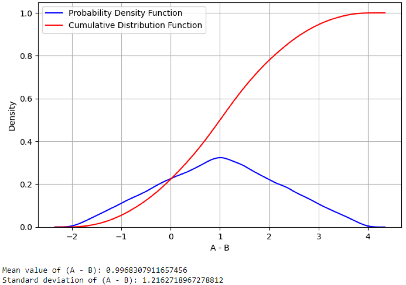
Monte Carlo simulation of A - B
#BackToBasics #CriticalThinking #MonteCarlo #ErrorAnalysis #Python