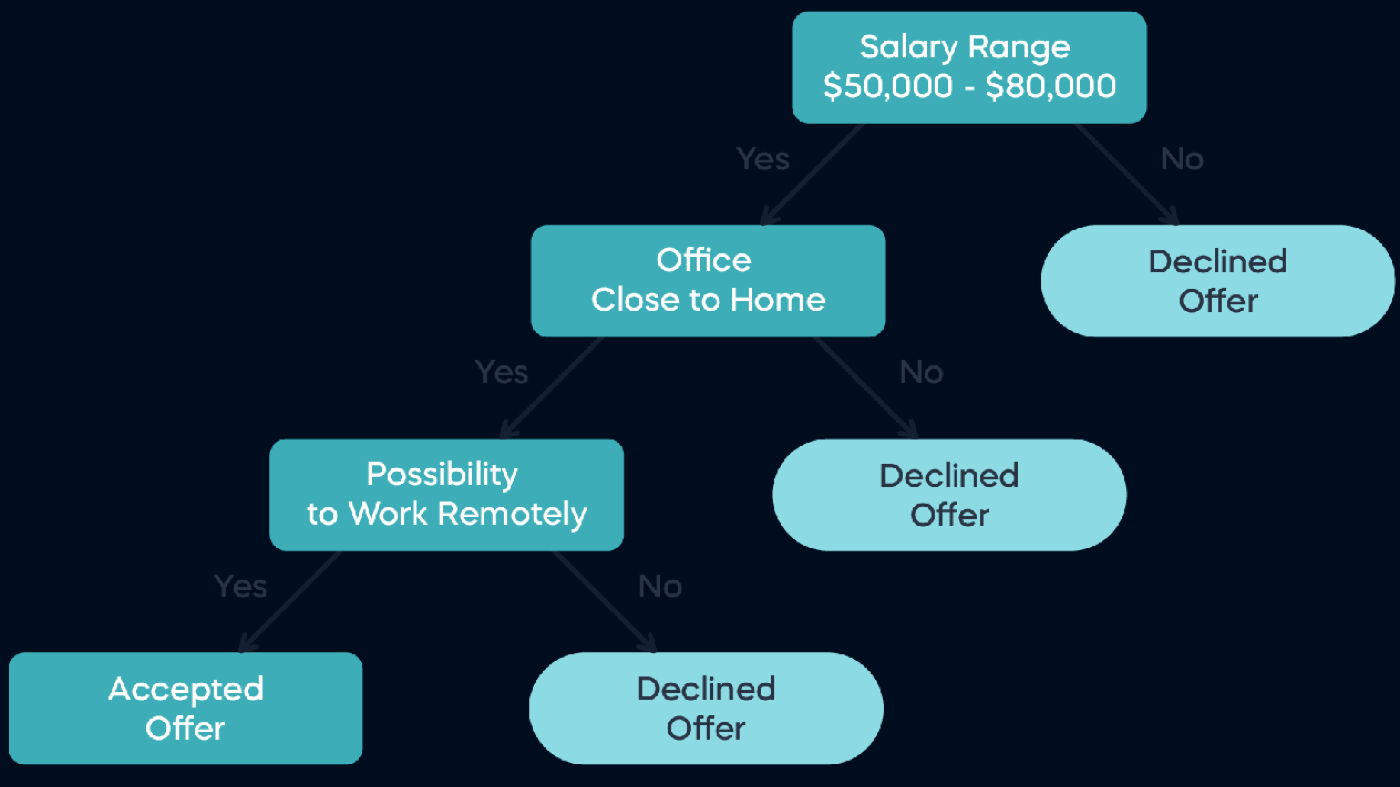
In my previous article on Discretisation vs. Monte Carlo, I touched on decision trees—but from the lens of decision analysis, where we model choices under uncertainty.
This article takes a different path. We’ll explore Decision Trees in Machine Learning (ML), a tool not for decision-making under risk, but for learning patterns from data.
Decision tree looks like below
🧠 What is a Decision Tree?
A Decision Tree is a model that learns decision rules from data. It works for both:
- Classification: “Will this well produce sand?”
- Regression: “What’s the expected flow rate given pressure and temperature?”
🌿 Anatomy of a Decision Tree
Understanding the structure helps explain how decisions are made:
- Root Node: The first question or split (e.g. “Is oil production > 1000 stb/d?”)
- Decision Node: An internal node that splits based on a feature (e.g. “Is water cut < 80%?”)
- Branches: The outcomes of a question (e.g. Yes → go left, No → go right)
- Leaf Nodes: The final output, a class label (e.g. “Choke up”) or a value
Each path from the root to a leaf is a decision rule.
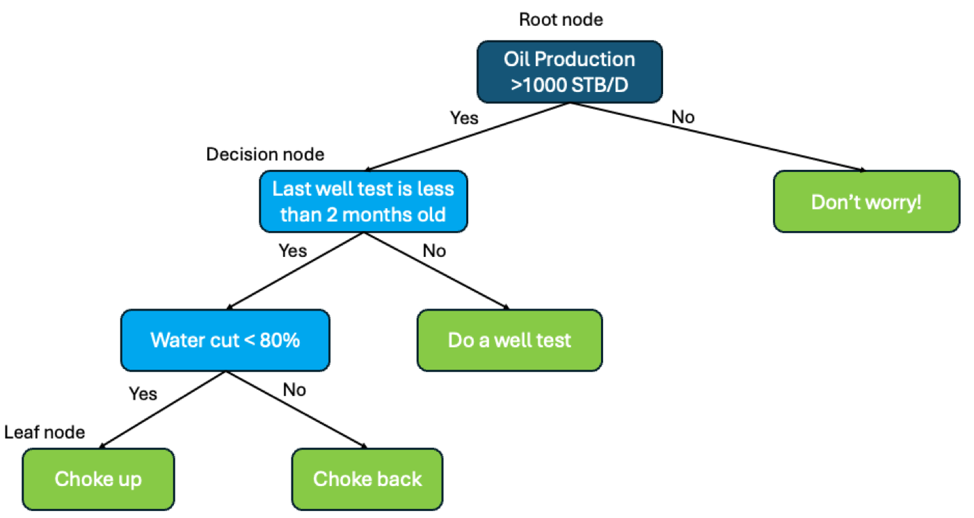
Just an example
📏 How Are Trees Built?
At each decision node, we look for the best feature/variable and threshold to split the data, using:
- Entropy or Gini Index for classification (how mixed the classes are)
- Mean Squared Error (MSE) for regression (how far predicted values are from actual)
We pick the split that gives us the most “information gain”, i.e. the biggest drop in uncertainty.
What’s “information gain”, you might ask? Let’s demonstrate with a little example of predicting Want to be PE variable as Yes or No based on the 3 variables, Love Math, Love Marvels and Age.
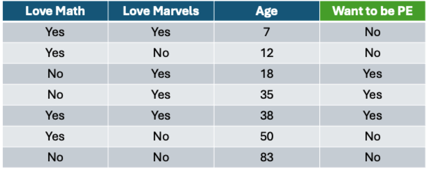
I should build a ML model to predict if any of my kids want to be a PE
🔶 Step 1: Start with a Mixed Bag
Suppose you have 7 balls:
- 🟢 = “Want to be PE: Yes” (3 balls)
- 🔴 = “Want to be PE: No” (4 balls)
This bag is fairly mixed → high uncertainty.
✂️ Step 2: Split by a Question (e.g. “Love Marvels?”)
Now, you divide the bag into two smaller bags:
- Left bag: Love Marvels = Yes → mostly 🟢 (Yes)
- Right bag: Love Marvels = No → only 🔴 (No)
✅ Step 3: Evaluate Purity
After the split:
- One bag is all red (pure No) 🔴🔴
- The other bag is mostly green (mostly Yes) 🟢🟢🟢🔴
That means the new groups are less mixed than the original.
→ This reduction in “mixing” is Information Gain.
💻 Python in Practice
Here’s how you’d build and evaluate a regression tree in Python:
Use case: Predicting oil rate from pressure, temperature, and water cut.
Bonus: You can even visualise the tree to see how decisions are made.
🎯 Enter Ensembles: Bagging and Boosting
Single decision trees are prone to overfitting because they can memorise the training data, especially if grown deep with many splits. To solve overfitting and boost accuracy, we combine multiple decision trees.
🌲 Random Forest (Bagging)
- Trains many trees in parallel on random samples of the data
- Reduces variance by averaging predictions
- Great for noisy sensor data, like from SCADA or downhole gauges
🔁 Gradient Boosting
- Builds trees sequentially, each focusing on correcting the previous tree’s mistakes
- Reduces bias and improves accuracy
- Very effective in problems like forecasting ESP failures or gas lift optimisation
🛢️ Oil & Gas Use Cases
Here are a few ways ML decision trees are applied in our industry:
🧪 Classification Tree
Predicting if a well is experiencing production impairment based on flow rate, tubing pressure, and historical trends.
⚙️ Regression Tree
Estimating daily liquid production from choke size, temperature, and casing pressure.
🌲 Ensemble Methods
Forecasting decline trends or classifying sand-producing wells across large well portfolios.
✅ Why Engineers Like Trees
- Transparent and explainable (no black boxes)
- Naturally handle missing values and different data types
- Can be exported as rules for automation or field deployment
🚀 Final Thoughts
While decision trees in decision analysis help us make choices under uncertainty, ML decision trees help us uncover data-driven patterns and predictions.
They’re different tools, from different disciplines, and both have their place.